For those who have been reading along with my past couple of blog posts, you’ve seen me explore different means of utilizing computational modeling to explore epidemic dynamics. In my last two posts (here and here), I developed a basic set of scripts (in R and Python) which apply a series of simple formulae to model aggregate/bulk infection dynamics in a population. In this case, the model is considered deterministic: meaning that my outcome will be the same every time I run the model.
Now, these mathematical/deterministic models can be useful for approximating the general outcomes of an outbreak, however they can fail to capture the nuances which might be present in a more complicated model. There is less flexibility in this kind of model to alter population or disease behaviours without completely redefining our equations. This is not to say that such models cannot be created, simply that I do not have the expertise or know-how to do so.
Instead, since the beginning of this project, my intention has been to utilize agent based modeling (ABM) as a tool for exploring epidemic dynamics. Just to restate what I discussed in this post, an agent based model does not utilize formulas to model epidemics; instead, the modeler must design agents (objects in an artificial/simulated world), define how these agents interacts, and when they interact. The simulation is then run, and the outcome determined at the end. Typically, these simulations incorporate some degree of randomness, so no two simulations will have exactly the same results (provided the random number generator seed is different).
Jordan’s First ABM
I decided to start simple for my first attempt at designing an ABM, though I did not want the model to be so simple that it would no longer be meaningful. There are three major components to any agent based model, and I will try to describe how I implemented each part in my model. I define each of the components of my model as a Python class for ease of use, and efficiency of code:
- Environment: In order for an ABM to exist, there must first be a space in which our agents can exist and interact. In my model, I call this the “World” class, and take this world to be a spatially homogenous region in which social beings can interact. Though the world I use is simplistic (possessing no geographic traits or barriers), it will serve well for this initial model. In future models, I hope to simulate a more realistic world, perhaps using GIS data from a major city (like my current home, Houston), in order to account for spatial factors in disease transmission.
- Agents: In this case, there are two major types of agents, hosts and pathogens. I’ve defined my hosts under the “Person” class, though really they are too simplistic to accurately represent people (they just interact with one another, not the environment); instead it may be helpful to think of them more like any other social organism. The pathogens, on the other hand, are defined by the “Disease” class; they are simply capable of infecting hosts, adding an “Infection” class to be stored in for a given host (this class contains the logic for recovery and death of the host).
- Relationships: In order for anything to happen in the simulaton, relationships must be defined in order to dictate how the various agents interact with one another. I’ve used my limited knowledge of graph theory to define a network of social interactions between various members of the “Person” class. I use the networkx Python library to generate this graph. Each of the nodes in the graph represent a person, and the edges represent a social connection (the two nodes/hosts know one another and regularly interact). I utilize a randomly generated, small world network topology to simulate a semi-realistic social network. If all this graph theory, mumbo-jumbo doesn’t make a lot of sense to you, read on, I’ll try and explain it more in the next section.
A Quick Primer on Graph Theory
The name “graph theory” is actually a bit deceptive, because it does not refer to the kind of graphs that we typically think of: those with an X and Y axis which depict the relationship between different variables. Instead, graph theory describes the relationships between different entities. These graphs look like spider-webs or clouds of points connected together by various lines. There are two parts to any graph: nodes, the points on a graph which represent the interconnected entities; and edges, the lines which connect nodes on the graph.
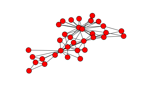
An example graph, depicting the relationships between various members of a university karate club. Generated by networkx, using karate_club_graph()
Small World Networks
Previously, I mentioned that I am utilizing a small world network in my model. This term may seem a bit daunting, but describes a familiar concept. I can frame it best in terms of the idea of six degrees of separation, which suggests that in real-world human social networks, any one typical individual is socially connected to any other by a chain of relationships between no more than 6 people. Human society is large (there are a lot of people, and a lot of space) and complex, so this idea may initially seem difficult to believe, but it makes sense in light of a simple principle. There are certain individuals who are able to span long-distances in a given population; these are the individuals who are capable of connecting far-off individuals to one another. For instance, you may live in New York, but have a cousin in California who is able to connect you to any number of people on the opposite side of the country (maybe even a Hollywood celeb).
A small world network mirrors this simple idea. While many nodes (individuals) are connected only to those close by, there are some nodes which have connections that can span great distances to reach far away parts of the network. In this way, most of the nodes are fairly well connected to one another. One counterintuitive aspect of graph visualizations (like the one above) is the fact that the position of each node does not matter for the determination of distance between two nodes; in fact, the nodes are initially placed randomly on an x/y plane for visualization purposes. Instead, distance in graphs is measured by the minimum number of edges (the lines between nodes), needed to travel from one node to another. Small world networks minimize this distance for any two given points.
Creating a Small World Network
While the algorithms for generating a small world network may seem complicated, they can be boiled down to a simple approach. First, we generate a regular network (one in which nodes are only connected to those close by to them). We then randomly select nodes and “rewire” them, connecting them to a distant node. This process can be visualized below in a plot from a 1998 Nature publication on the subject by Watts and Strogatz.
Concluding Thoughts
This article has gotten a bit longer than I originally expected. I’m gonna end it here, and pick up next time with a review of the results from my first ABM simulation. Thanks for reading!